Extracting Data from a Concatentated String in Excel

Published: 5 February 2018

Excel. The multi-tool in every BA's tool-belt. Or if it's not, it should be.

From capturing user stories, calculating cost basis, data analytics, metrics tracking, management dashboards, and it's default use as the table-creation-tool du-jour; it does it all. It may not be the BEST tool for any of those but it's the tool you can count on almost everyone in an office environment having and being at least somewhat familiar with.

It's also the tool that most people I know turn to when you get one or more data dumps of some sort and you need to try and make sense of the information, or just make it more accessible for further analysis.

In this post I am going to discuss a specific problem I encountered with a data extract in the form of an Excel file. That problem was that:

Out of about 25 data elements in the file, only about 10 were in distinct columns
The rest of the data elements were concatenated together into one string in a single column
There were nearly a thousand rows of data and I would be getting a new file every month, meaning a manual solution was not desirable
The discreet data values in the string were not always consistently present (e.g. a value might be present in one row but not another)
The data values in the strings were not always in the same order

So in this post I am going to go through the logic and eventual Excel functions that were created to solve this problem. Hopefully you find it useful.

The Data

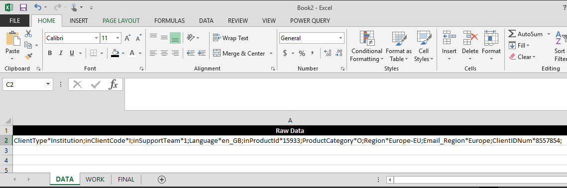
In the case I faced the actual concatenated looked like this, with data labels attached to every data element in the string. The string below uses the same structure as the actual data set I received at work except that I changed the actual labels and values:

ClientType*Institution;inClientCode*I;inSupportTeam*1;Language*en_GB;inProductId*15933;ProductCategory*O;Region*Europe-EU;
    Email_Region*Europe;ClientIDNum*8557854;

As you can see, the data is semi-colon delimited, includes a data label for each distinct value, and the data values are not always going to be the same consistent length (for example, a Region value might be Europe-EU, Europe-NonEU, USA, or similar variable lengths).

The Problem

The main problem with this data set was that all of the data elements are not always present or sometimes they might be located in different parts of the string. This means that there is no consistent order of the elements in the string and if you want to extract the data you need to identify the values by label, not by location.

So how would you go about extracting each individual data element from that string into its own cell? I am going to walk through an example of what I actually did in this scenario, not just showing the formulas but how I built them and the logic that led me to certain solutions. Hopefully you find it useful.

As a refresher, here's the data example again. This time in an actual Excel workbook:

In that single cell there are the following individual data values that I needed to extract:

Client ID Number
Client Type
Client Code
Support Team
Language Code
Product ID
Product Category Code
Client Region (identified as just 'Region')
Email Region

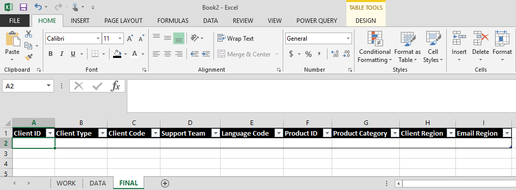
Given that I know I will be getting a new extract every month, my plan was to create a 'DATA' worksheet that I would copy the extract to, a 'WORK' worksheet that would contain any supplemental information I needed, and a 'FINAL' worksheet that would have the cleaned up data set.

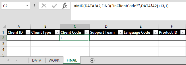
And for simplicities sake, in this explanation I am going to assume that the concatenated string is my only column of data and that I want to extract those elements to columns A through I, starting in Row 2, with Row 1 being column headers. The image below shows the start of my 'FINAL' worksheet.

Showing My Work

To build an Excel function that will pull out a single piece of information from the 'DATA' worksheet, let's think about what we need to happen and build the formula from outside in.

Step 1 - Identifying the Main Function

First of all, we need to understand what function is going to achieve our primary goal. Given our scenario, our primary goal is that we want to extract a sub-string of text from the overall text string. We know each sub-string will not always be at the beginning or end of the main string, so we don't want to use the LEFT or RIGHT functions in Excel. Rather, we want to use the MID function.

As the linked Microsoft page states, MID returns a specific number of characters from a text string, starting at the position you specify, based on the number of characters you specify.

The syntax for MID is:

MID(text, start_num, num_chars)

text - Required. The text string containing the characters you want to extract.
start_num - Required. The position of the first character you want to extract in text. The first character in text has start_num 1, and so on.
num_chars - Required. Specifies the number of characters you want MID to return from text.
num_bytes - Required. Specifies the number of characters you want MIDB to return from text, in bytes.

We know the text string we want to extract from is located at [DATA!A2], but we don't know where one of our desired sub-string starts or how many characters we want to extract. That means that our formula right now looks like this (with the question marks indicating unknown elements of the formula we still have to solve for):

=MID(DATA!A2,?,?)

Step 2 - Finding the beginning of the sub-string

To add the next required element of our MID formula, we need to know the character number in our base text string from which we want to start extracting our substring. To do this we want to use the Excel FIND function.

As the linked Microsoft page states, FIND and FINDB locate one text string within a second text string, and return the number of the starting position of the first text string from the first character of the second text string.

The syntax for FIND is:

FIND(find_text, within_text, [start_num])

find_text - Required. The text you want to find.
within_text - Required. The text containing the text you want to find.
start_num - Optional. Specifies the character at which to start the search. The first character in within_text is character number 1. If you omit start_num, it is assumed to be 1.

NOTE that you could also use the SEARCH function which is like FIND except that SEARCH is not case sensitive while FIND is case sensitive. While FIND is thus easier to mess up if you don't get the capitalization of your search term correctly, I find it more accurate.

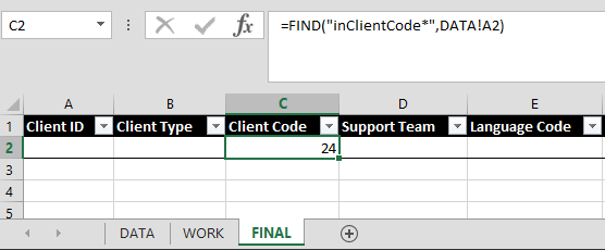
So given that, if I want to extract the value of the Client Code element in the data, I would start with this:

    =FIND("inClientCode*",DATA!A2)

In the example data set above this would return a value of 24 since the start of the sub-string inClientCode* is the 24th character within the larger string located in cell A2. You can see this in the image below where I have plugged the formula into my spreadsheet.

If we take this information and nest the FIND function within the MID function, our function currently looks like this:

    =MID(DATA!A2,FIND("inClientCode*",DATA!A2),?)

However, I don't actually want to start extracting my sub-string with the beginning of the inClientCode* label. Rather, I want to start extracting after the label and separator (the asterisk). So I count the number of characters from the beginning of inClientCode* to where I do want to start my extract. Since there are 13 characters in inClientCode* I want to add 13 characters to the starting location my formula, which makes it look like this:

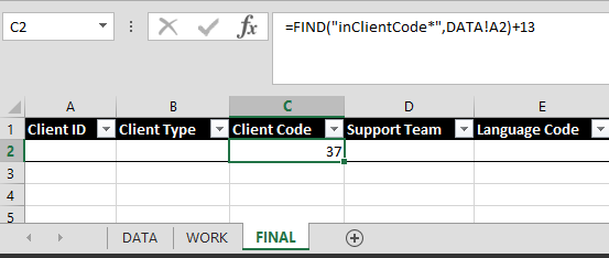
When I add that formula to the main MID function, it now looks like this:

    =MID(DATA!A2,FIND("inClientCode*",DATA!A2+13,?)

Step 3 - Finding the end of the sub-string

Our main function is now just missing just one more piece of information, and this is the number of characters we want to extract beginning at the starting location we identified in the previous step.

If the information you want to extract is always the same length, such as a single character, this is easy and you can just put that value in the formula. For example, I know my Client Code, Support Team, and Product Code values in the data set are always 1 character long. Thus I can just enter 1 into my formula and I am done for those data elements. My completed formula would look like this:

    =MID(DATA!A2,FIND("inClientCode*",DATA!A2)+13,1)

And as shown below when I enter that into Excel it returns just the actual Client Code value of I:

But as you can see from the other data elements in our sample string, you may not have a fixed-length value. And unfortunately, this is where things start to get complicated.

In theory, you could use the 'start_num' argument of the FIND function to have the FIND function start where your element label starts. But to do that within a single function you would need to have a FIND argument within another FIND argument (the 2nd to find your label start) and Excel doesn't allow this.

You also can't use a similar Excel function like SEARCH within a FIND function. You CAN have more than one FIND function within a parent function (such as our MID), but that won't solve our problem with this potential solution of being unable to nest one FIND within another. So if you can't nest a FIND within another FIND or SEARCH, what are your options?

A SUBSTITUTE option?

If you knew that your all of your data elements were always present and in the same order, you could use the SUSTITUTE function like this (if the Region element was always the 8th element in the string):

    =MID(DATA!A2,FIND("Region*",DATA!A2)+7,(FIND(CHAR(160), SUBSTITUTE(DATA!A2,";",CHAR(160),8)))-(FIND("Region*",DATA!A2)+7))

This only works if I know that the Region element is always going to be present and will always be the 8th value in the string. So I am telling Excel to first FIND starting point as I did above (the [FIND(Region*,DATA!A2)+7] part). Then I am using the SUBSTITUTE function to change the 8th instance of the semi-colon character into a special character [CHAR(160)] that in most cases should not be present in the data. I embed that SUBSTITUTE function within a FIND function to identify the end location of my sub-string, and then subtract the result of another FIND function that locates the start of my sub-string to give me the length value.

Note that there are three distinct FIND functions within the MID function, all of which are distinct and which don't need another FIND to resolve. Unfortunately, this potential solution won't work in my scenario because I know that values aren't always present in every row (meaning that Region* may not even be in the my string) and that they aren't always in the same location (so I can't know to SUBSTITUTE the 8th semi-colon since that may not be the one associated to Region).

This meant I could not use SUBSTITUTE and had to find another solution.

The 'Pointers' Solution

The solution I eventually found was why I added the 'WORK' worksheet to my Excel file and actually results in simpler formulas. The solution was to essentially perform a nested FIND in two different steps, in two different locations.

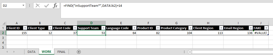
What I did was to take the FIND function that identifies the start of the data I want to extract, and place the results of the function on the WORK tab. These would act as 'Pointers' to my starting point and give me a discreet value outside of my main formula that I can refer to. It also pulls the FIND needed to identify that location out of my main formula.

The image below shows the WORK tab with the table of pointers of set up. I also added a FAKE element to the table below so that you can see that when a match is not found Excel returns an error code.

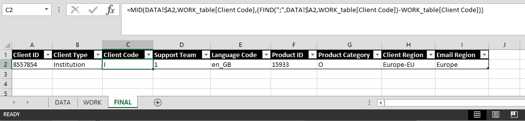
Now I don't have to worry about nested FIND functions. Rather, I use the WORK table with its dedicated FIND functions to locate the start of each data value. Then on the FINAL tab I just point to the appropriate cell in the WORK table to get the starting location I need for my MID function, and to supply the value I need to subtract from the remaining FIND function to determine the number of characters I want the MID function to extract.

The result is a formula that looks like the image below:

The last thing to consider is how to handle rows where the data element you are looking for is missing. What that happens the formula will return a #VALUE error as shown in the FAKE column above. The way to handle this is with the Excel IFERROR function.

The IFERROR function Returns a value you specify if a formula evaluates to an error; otherwise, returns the result of the formula. And its syntax is:

    IFERROR(value, value_if_error)

value - Required. The argument that is checked for an error.
value_if_error - Required. The value to return if the formula evaluates to an error. The following error types are evaluated: #N/A, #VALUE!, #REF!, #DIV/0!, #NUM!, #NAME?, or #NULL!.

So if I want to replace an error with a null string, I would use the following formula:

    =IFERROR(MID(DATA!A2,WORK_table[Client Code],FIND(";",DATA!A2,WORK_table[Client Code])-WORK_table[Client Code])),"")

If you want to change the default value on error to something else, just put that something between the double-quotes at the end.

Wrap-Up

Well, that's it. I had to learn the hard way about nested FIND functions, so the solution shown above came about after several hours of frustration. But it's given me a workable solution for this situation in the future. And the SUBSTITUTE option discussed above works when I have consistent data elements in a consistent order.

I hope you find this useful as both a solution and as a learning opportunity on Excel functions.

Best wishes.